Least Squares

Applications of Least Squares

One of the most important applications of the least squares is data fitting.

Suppose we are studying a certain phenomenon, which can be schematically represented as follows:

Pasted image 20231025050855.png

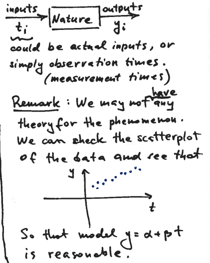
Let $(t_{1}, y_{1}), \dots, (t_{m}, y_{m})$ be the collected data. Suppose that the theory underlying the phenomenon indicates that $y = α + β t$

Goal: To find $α$ and $β$ from the data $(t_{i}, y_{i})$
Simple example: An object is moving with a constant speed $β$ and at time $t = 0$ its position was $α$ . $\Rightarrow$ at time $t$ its position is $y = α + β t$ .

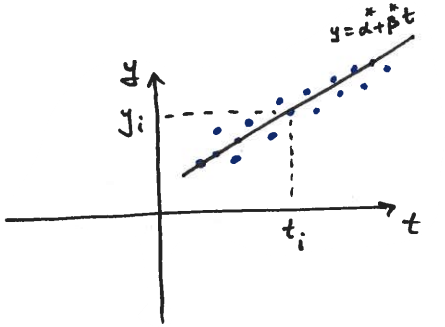
In an ideal world, where the theory is absolutely correct (i.e. exactly describes the phenomenon) and there are no measurement errors, $y_{i} = α + β t_{i}$ for all $i = 1, \dots, m$ and just two data points tare enough to compute $α$ and $β$ .

In reality, even if the linear model is correct, the data looks like this:
Pasted image 20231025051653.png
(measurement errors are inevitable) $\Rightarrow$ there is no line that goes exactly through all data point

Goal: To find a line $y = α^{*} + β^{*} t$ that "fits best" the measured data and use $α^{*}$ and $β^{*}$ as the estimates for $α$ and $β$ .

Question: What does it mean "fits best"?

There are several ways to define the best fit, here is one:
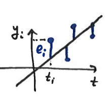
The difference between the observed value $y_{i}$ and the value predicted by the model is called the residual (also called prediction error in engineering fields): $e_{i} = y_{i} - (α + β t)$ . Let $e = (e_{1}, \dots, e_{m})^{T}$ be the vector of residuals. $[\begin{matrix} e_{1} \\ ⋮ \\ e_{m} \end{matrix}] = [\begin{matrix} y_{1} \\ ⋮ \\ y_{m} \end{matrix}] - [\begin{matrix} 1 & t_{1} \\ ⋮ & ⋮ \\ 1 & t_{m} \end{matrix}] [\begin{matrix} α \\ β \end{matrix}]$
We would want all residuals to be small. The overall measure of the fit is the Euclidean norm of $e$ . Thus, we are looking for the coefficient vector $x^{*} = (α^{*}, β^{*})^{T}$ that minimizes the Euclidean norm of the residual vector.

x^{*} = a r g m i n_{x \in R^{2}} | | A x - y | |_{2} = | | e | |_{2}

Geometrically:
Pasted image 20231025052539.png

But this is exactly the least squares solution to the system $A x = y$ .

Remark: In principle, we can minimize $| | e | |_{1} = | e_{1} | + \dots + | e_{m} |$ or $| | e | |_{α} = m a x {| e_{1} |, \dots, | e_{m} |}$ , but these minimization problems are much harder, nonlinear, and to solve them, we need to use tools outside of linear algebra. As a result of simplicity, least squares is used in most applications.

Last time we established the following result: if $k e r A = {0} \Rightarrow x^{*} = (A^{T} A)^{- 1} A^{T} y$ . In our case, $A = [\begin{matrix} 1 & t_{1} \\ ⋮ & ⋮ \\ 1 & t_{m} \end{matrix}]$ . Therefore, $k e r A = {0} \Rightarrow$ columns of $A$ are linearly independent $\Rightarrow$ not all $t$ ; are equal (a very weak assumption). Basically, we need to measure $y$ at least two distinct times (or two distinct points).

Under assumptions that not all $t_{i}$ are equal:

A^{T} A = \begin{matrix}  \end{matrix}

This system of two equations is easy to solve:

α^{*} = \bar{y} - \bar{t} β^{*}, β^{*} = \frac{\bar{t y} - \bar{t} \bar{y}}{\bar{t^{2}} - (\bar{t})^{2}} = \frac{\sum (t_{i} - \bar{t}) (y_{i} - \bar{y})}{\sum (t_{i} - \bar{t})^{2}}

Thus, the best -- in the least squares sense -- straight line that fits the given data $(t_{y}, y_{i}), i = 1, \dots, m$ is $y = α^{*} + β^{*} t$ .

Remark: Often problems that don't look like linear least squares problems can be converted to the least squares formulation by taking appropriate transformations of participating variables.

Let $m_{i}$ be the (measured) amount of radioactive material in a sample of an unknown isotope at time $t$ ; Data: $(t_{i}, m_{i})$ . Theory $m (t) = m_{0} e^{β t}$ , $m_{0}$ initial mass, $β < 0$ decay rate. Problem: find $m_{0}$ and $β$ . The model is not linear, but: $\log m (t) = \log m_{0} + β t$ . We can fit this to $D = (t_{i}, \log m_{i})$ .

Suppose the scatterplot of the data $(t_{i}, y_{i})$ looks like this:
Pasted image 20231025055222.png

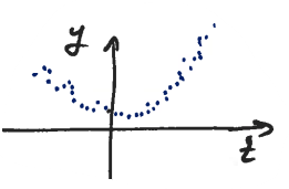
We can fit a line to the data, but it does not really make sense. A parabola $y = α + β t + γ t^{2}$ seems to be a better model. In general, suppose we want to fit a polynomial of degree $n$ to the data
$y (t) = α_{0} + α_{1} t + \dots + α_{n} t^{n}, α_{i} \in R$
The $i$ th residual: $e_{i} = y_{i} - y (t_{i}) = y_{i} - (α_{0} + α_{1} t_{i} + \dots + α_{n} t_{i}^{n})$ , $i = 1, \dots, m$ .
$[\begin{matrix} e_{1} \\ ⋮ \\ e_{m} \end{matrix}] = [\begin{matrix} y_{1} \\ ⋮ \\ y_{m} \end{matrix}] - [\begin{matrix} 1 & t_{1} & \dots & t_{1}^{n} \\ 1 & t_{2} & \dots & t_{2}^{n} \\ ⋮ & ⋮ & \dots & ⋮ \\ 1 & t_{m} & \dots & t_{m}^{n} \end{matrix}] [\begin{matrix} α_{0} \\ ⋮ \\ α_{n} \end{matrix}]$
$A$ is called a Vaudermoude matrix (French mathematician that did not introduce the Vandermonds matrix) $A \in M_{m \times (n + 1)}$ .

Consider a special case: $m = n + 1$ (# measurements = # coefficients) $\Rightarrow$ $A$ is square and, if $A$ is nonsingular, we can find $x$ such that $e = 0$ . In other words, we can solve $A x = y$ exactly, i.e. find a polynomial that fits the data ${(t_{i}, y_{i})}$ exactly. This polynomial is called interpolating polynomial.

Lemma: If $t_{1}, \dots, t_{n + 1}$ are all distinct $(t_{i} \neq t_{j})$ $\Rightarrow$ the $(n + 1) \times (n + 1)$ Vandermond matrix is nonsingular.

Remark: Textbook gives a proof based on an LU decomposition. But the statement is very intuitive if you think about it geometrically.